Three-of-a-kind
Table of Contents
1 Rules of the game
A post on the Mathematics Stack Exchange (https://math.stackexchange.com/questions/1854082/variable-triples-vs-single-quad-card-game-who-has-the-advantage) poses the following question:
Suppose we start drawing cards from a standard playing card deck, putting them in a pile. We'll say the pile has a triple in it if any three cards have the same face value (e.g. QQQ), and a quartet if any four cards have the same face value (e.g. 3333). The order of the cards doesn't matter, so for example the pile [A, 3, 8, A, 1, A] contains a triple of aces, even though the aces aren't consecutive.
We'll continue drawing until either the pile contains a quartet—in which case you win the round—or the pile contains four different triples—in which case I win the round.
After the round is over, we return all cards to the deck, shuffle, and play another round—except we adapt the difficulty level: if I won last time, we increment the number of triples I need in order to win. If I lost last time, we decrement the number of triples instead.
Question: In the long run as we play many rounds, does this game approach an "equilibrium difficulty level" of some kind? That is, does the game converge on a difficulty level where you and I are approximately equally likely to win?
2 A splendid solution
One approach to this problem is to play (or simulate) many rounds of this game yourself in order to discover whether the game tends toward equilibrium. Another solution is to compute the various probabilities involved to discover the answer numerically . But it turns out the question has a beautifully succinct conceptual answer!
Notice that the game has the following three properties:
- Adaptability
- The difficulty of the game — that is, the probability that I win the next round — increases whenever I win and decreases whenever I lose.
- Zero-sum
- Exactly one of us wins each round. (Thus, the more likely I am to win, the more likely you are to lose.)
- Straddling
- At some level of difficulty, I am more likely to win than lose. At another, I am more likely to lose than win.1
Now suppose we make a list of the possible game difficulty levels, ranging from \(n=1\) to \(n=14\).
| 1 | 2 | 3 | 4 | 5 | 6 | 7 | 8 | 9 | 10 | 11 | 12 | 13 | 14 |
I want to divide these into levels where I am more likely to win and levels where I am more likely to lose. Except for \(n=1\) (guaranteed win) and \(n=14\) (guaranteed loss), I don't know the exact probabilities — but I do know that because the game gets progressively more difficult, all of the most-likely-win states must be on the left, and all of the most-likely-lose states must be on the right.
But this means that whenever the game is in the "left" group, it will tend to progress rightward, and whenever the game is in the "right" group, it will tend to progress leftward! Hence we can conclude that the game will reach equilibrium—at the interface between the most-likely-win and most-likely-lose states, wherever that is. In other words—
Yes, the game must always converge toward an equilibrium state. (And so must any similar game which has the adaptability, zero-sum, and straddling properties!)
3 Further investigations
3.1 Using symmetry to count cards quickly
But what is the equilibrium difficulty level? If we knew my win probability for each difficulty level, we could simply locate the level where the probability switches from being less than ½ to greater than than ½.
More generally, how can we compute the probability that we will draw \(n\) triples before we draw one quartet? For some difficulty levels \(n\), the probability is easy to calculate by hand because it is trivial \((n=0, n=14)\). And in a few other cases, we can use clever conceptual tricks to compute the probability with only slightly more difficulty.
For example, when \(n=13\): drawing 13 triples before drawing a single quartet is equivalent to drawing thirteen cards with distinct faces from the back of the deck. (This is because those thirteen cards are the missing pieces of the quartets in the beginning of the deck.)
So we have that for \(n=13\), my probability of winning is:
$$\frac{52}{52}\times\frac{51-3}{51}\times\frac{50-6}{50} \times \ldots \times \frac{52-4k}{52-k}\times\ldots \times \frac{4}{40}$$ which is a probability of around 0.0001.
But besides these few easy cases, it seems that the probability calculations are rather involved. (For \(n=2\), what is the probability of drawing two triples before drawing a quartet?) Part of the difficulty stems from the fact that we must keep track of so many different possible outcomes: you might draw two cards with the same rank first, or different ranks. With three cards, there are even more combinations, etc. Symmetry helps to cut down on some, but not all, of the work.
I considered writing a program to do the brute-force number crunching — but of course, there are \(52!\) different outcomes to consider, and so a naive algorithm would take an inordinate amount of time to run2. If only I could get a computer program to recognize the symmetry of various hands, I could write down a procedure for computing these probabilities while only considering outcomes that were essentially different from each other.
Here is a trick for consolidating symmetric situations: suppose we have a pile of cards drawn so far. We can tally how many cards of each rank we have, then arrange those tallies in order from biggest to smallest. For example, if our pile consists of:
| 5♠ | Q♣ | 3♦ | 5♦ | Q♥ | 2♦ |
We would note that we have 2 cards of rank 5, 2 cards of rank Q, and 1 card each ranked 2, 3, 5.
If we forget about the ranks and simply arrange the tallies from largest to smallest, we obtain:
| 2 | 2 | 1 | 1 | 1 |
Let us call this abstracted representation the tally form. Notice that the tally form has an essential property:
If two different piles have the same tally form, they also have the same probability of leading to a win condition.
This invariant "macrostate" representation leads to a straightforward algorithm for computing the probability of a win condition without too much combinatorial overhead. In Python-like pseudocode,
def WinProbability(n, deck, current_pile=[]) :
    if current_pile contains n triples :
        return 1
    elif current_pile contains at least one quartet :
        return 0
    else :

        let total_probability = 0
        let counts = new Dictionary()
        let representative_deck = new Dictionary()
        let representative_pile = new Dictionary()

        for each new_card in the deck :
            let new_deck = deck - new_card
            let new_pile = current_pile + new_card
            let tally = computeTally(new_pile)

            counts[tally] = counts[tally] + 1
            representative_deck[tally] = new_deck
            representative_pile[tally] = new_pile

        for each different kind of tally :
            total_probability += counts[tally] / length(deck) *
                                  WinProbability(n, representative_deck[tally],
                                                    representative_pile[tally])


        return total_probability
The actual Python source code is similar, although additionally I use a kind of memoization to cache computations that are performed repeatedly. (Thus the algorithm computes the win probability of each tally exactly once; if that tally is passed to the algorithm again in a later context, the probability is instead retrieved from memory.)
def compute_probabilities(n, deck, drawn=None) :
    # Compute the probability of winning (drawing n different triples
    # before the first quartet is drawn) given a deck and a list of
    # cards drawn so far.

    # Uses symmetry to reduce the number of cases. (This is the
    # purpose of the "canonicalize" function.)

    global memo

    # INITIALIZE
    has_quartet = lambda tally : any([k >= 4 for k in tally])
    has_n_triples = lambda tally : n <= len([k for k in tally if k == 3]) and not has_quartet(tally)
    drawn = drawn or []

    def remove(xs, x) :
        # nondestructively remove the first occurence of x from xs.
        ret = xs + []
        ret.remove(x)
        return ret

    def canonicalize(drawn) :
        # Abstract away from the specific cards and just look at the
        # number of cards from each rank.

        seen = {}
        for x in drawn :
            seen[x] = seen.get(x,0) + 1
        return sorted(seen.values())

    # BASE CASE: THE GAME IS OVER ALREADY
    representative = canonicalize(drawn)

    if has_n_triples(representative) :
        return 1
    elif has_quartet(representative) :
        return 0
    elif lookup(representative) :
        return lookup(representative)

    # RECURSIVE CASE: CONSIDER EACH ESSENTIALLY DIFFERENT DRAW
    unique_outcomes = []
    seen = []

    for card in deck :
        next_draw = drawn + [card]
        representative = canonicalize(next_draw)
        if representative not in seen :
            unique_outcomes += [(remove(deck, card), next_draw, representative)]
        seen += [representative]

    ret = []
    for next_deck, next_draw, representative in unique_outcomes :

        count = len([x for x in seen if x == representative])
        p = compute_probabilities(n, next_deck, next_draw)

        if lookup(representative) is None :
            memo += [(representative, p)]

        ret += [(count, p)]
    return sum([count * probability for count, probability in ret]) / float(len(deck))
This algorithm runs remarkably quickly — indeed, we can modify this algorithm slightly so that it will also report the number of recursive calls and/or calls to the memoization table. A naive algorithm would nominally need to consider all \(52!\) deck permutations and evaluate the winner of each. But here, in even the worst case ( when \(n=13\) ), the algorithm makes only 1820 calls to either itself or its memoization table — considerable savings!
We can now run this algorithm in a loop over all difficulty levels \(n=1,\ldots, 14\) to compute the probability that I will get \(n\) triples before the first quartet appears.
ranks = 13
deck = range(1,ranks+1) * 4

coords = []
r = 5
win_probability = [None] # probability of A winning at each level of difficulty
for n in range(1,ranks+1) :
    memo = [([],0)]
    p = float(compute_probabilities(n,deck))
    win_probability += [p]
win_probability += [0]
The data follows. In this table, I am "Player A", and you are "Player B". Of course, at each level of difficulty, \(P(A\text{ wins}) + P(B\text{ wins}) = 1\).
n       P(A wins)               P(B wins)
----------------------------------------------
1       1.0                     0.0
2       0.877143650546          0.122856349454
3       0.713335184606          0.286664815394
4       0.540136101559          0.459863898441
5       0.379534087296          0.620465912704
6       0.245613806098          0.754386193902
7       0.144695490795          0.855304509205
8       0.0763060803548         0.923693919645
9       0.0351530543328         0.964846945667
10      0.0136337090929         0.986366290907
11      0.00419040924575        0.995809590754
12      0.000911291868977       0.999088708131
13      0.000105680993713       0.999894319006
14      0.0                     1.0
From this table, a concrete answer to our conceptual question appears: yes, the game has an equilibrium—and the equilibrium lies between the states \(n=3\) and \(n=4\) (where the win probability switches between greater than ½to less than ½).
3.2 Evaluating rare outcomes with matrix math
Now that we have these numbers, we can compute some interesting quantities. Because this game has an attractor state near \(n=4\), we expect that most games will take place near difficulty \(n=4\). Furthermore, the question arises how many rounds we'd expect to play before ever reaching an unlikely difficulty level like \(n=13\) or \(n=14\). (How many steps do you think it will take?)
To answer this question, we will depict the game as a Markov process, where the difficulty levels of the game are represented as nodes ("states") in a graph, and arrows between the nodes denote the probability of the game transitioning from one level of difficulty to another.
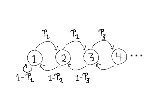
Every Markov process with \(n\) states can be represented as an \(n\times n\) matrix \(P\), where the entry \(P_{ij}\) denotes the probability of transitioning from state \(i\) to state \(j\). According to the rules of this game, of course, the difficulty level only increases or decreases by one each round, and so \(P_{i,j} = 0\) unless \(j=i+1\) or \(j=i-1\).
Borrowing from the theory of Markov processes, we find the following result:
Markov expected-length calculation: If you have a Markov process represented by an \(n\times n\) matrix \(P\) and you want to compute the expected number of steps it will take to get from state \(i\) to state \(j\), you can do so as follows:
- Let \(\vec{\mathsf{ones}}\) be an \((n-1)\times 1\) column vector where each entry is 1.
- Define \(Q \equiv I_n - P\). Here, \(I_n\) denotes the \(n\times n\) identity matrix.
- Delete row \(j\) and column \(j\) from \(Q\).
- Solve the matrix equation \(Q \cdot \vec{x} = \vec{\mathsf{ones}}\) for the unknown vector \(\vec{x}\).
The entires of the solution \(\vec{x}\) will be the expected number of steps to reach node \(j\) from the various other states. (Note that the expected number of steps to reach node \(j\) from itself is 0, and that this entry is not included in \(\vec{x}\) ).
\(\vec{x} = [E_1, E_2, \ldots, E_{j-1}, E_{j+1}, \ldots E_n]\).
The expected number of rounds to get from difficulty 4 to ...

    ... difficulty 1 is 150 rounds.
    ... difficulty 2 is 22.11 rounds.
    ... difficulty 3 is 5.34 rounds.
    ... difficulty 4 is 0 rounds (already there.)
    ... difficulty 5 is 3.48 rounds.
    ... difficulty 6 is 11.81 rounds.
    ... difficulty 7 is 41.46 rounds.
    ... difficulty 8 is 223.65 rounds.
    ... difficulty 9 is 2,442 rounds.
    ... difficulty 10 is 63,362 rounds.
    ... difficulty 11 is 4,470,865 rounds. (over 1 million.)
    ... difficulty 12 is 1,051,870,809 rounds. (over 1 billion.)
    ... difficulty 13 is 1,149,376,392,099 rounds. (over 1 trillion.)
    ... difficulty 14 is 12,354,872,878,705,208. (over 10 quadrillion.)
from numpy import array
from scipy.linalg import solve

 # ---------- EXPECTED NUMBER OF ROUNDS
  ranks = 13

  # The vector of win probabilities for me at difficulty levels
  # n=1,2,3,..,14.  I want to use one-based indexing, so ps[0] is None
  # (unused.)
  ps = [None, 1.0, 0.8771436505456077, 0.713335184606418, 0.540136101559028, 0.3795340872959987,
       0.24561380609752134, 0.1446954907949892, 0.07630608035483175, 0.03515305433278668,
       0.013633709092936501, 0.004190409245747548, 0.000911291868976561, 0.00010568099371338212, 0]


  for absorb in range(ranks+1) :
      P = [[
          -1* (-1 if i ==j else 0 if abs(i-j) != 1 else ps[j] if j > i else 1-ps[i+1])
          for j in range(ranks+1) if j != absorb]
           for i in range(ranks+1) if i != absorb]

      ones = array([[1] for i in range(ranks)])
      m = solve(array(P), ones)
      print absorb+1, int(m[3 if absorb >= 3 else 2])
3.3 Exponentials predict where you will end up
If you play (or simulate) several rounds of this game, you may notice that the game reliably maintains its equilibrium, staying near difficulty level \(n=4\). To put it another way, this game reliably ensures that you and I win approximately the same number of rounds.
(One neat observation to think about is that this game reaches difficulty level \(n\) just if I have won \(n-4\) more games than you have.)
For exploration's sake, we might compare the outcomes of this game against the outcomes of tossing a theoretical fair coin. Like this game, a repeatedly-tossed fair coin is expected to come up heads around as often as it comes up tails. But our game is adaptive, whereas (contrary to the gambler's fallacy) a fair coin has the same probability of coming up heads regardless of its history. (Fair coins are "memoryless".) Because our game adapts to encourage fairness, we should expect a sequence of rounds in this game to be even more reliably fair in the long run than an equivalent sequence of fair coin tosses.
We can evaluate the probability of using the powers of our transition-probability matrix \(P\), which we defined in the previous section. Indeed, for any power \(k\) the matrix \(P^k\) describes where we are likely to be after \(k\) turns, depending on where we started. To be specific, each entry \(P^k_{i,j}\) gives you the probability of being in state \(j\) after \(k\) moves, having started in state \(i\).
[0, 0.126, 0, 0.599, 0, 0.262, 0, 0.011, 0, 0, 0, 0, 0, 0] # even rounds
[0.015, 0, 0.386, 0, 0.521, 0, 0.075, 0, 0, 0, 0, 0, 0, 0] # odd rounds